ML - Distance Metrics

Goal¶

To visualize how each metric works and compare them.

Introduction¶

Distance metrics measure how far apart two data points are. They’re fundamental to many ML algorithms like KNN, K-Means clustering, and similarity searches.

we’ll explore:¶

Euclidean Distance - straight-line distance
Manhattan Distance - grid-based distance
Minkowski Distance - generalized distance
Cosine Distance - angle-based similarity

Setup: Import Libraries¶

import numpy as np
import matplotlib.pyplot as plt
import seaborn as sns
from scipy.spatial.distance import euclidean, cityblock, cosine, minkowski
from sklearn.metrics.pairwise import euclidean_distances, cosine_distances

# Set style for better visualizations
sns.set_style('whitegrid')
plt.rcParams['figure.figsize'] = (12, 8)

print("✓ All libraries imported successfully!")

✓ All libraries imported successfully!

1. Euclidean Distance¶

Formula¶

The straight-line distance between two points. Like measuring distance on a map with a ruler.

d(p, q) = \sqrt{(p_1 - q_1)^2 + (p_2 - q_2)^2 + \cdots + (p_n - q_n)^2}

(1)

Characteristics¶

Most common distance metric
Assumes you can move diagonally
Sensitive to all dimensions equally
Good for most ML tasks

# Example: Calculate Euclidean distance
p = np.array([0, 0])
q = np.array([3, 4])

# Method 1: Manual calculation
dist_manual = np.sqrt((p[0] - q[0])**2 + (p[1] - q[1])**2)

# Method 2: Using scipy
dist_scipy = euclidean(p, q)

print(f"Point P: {p}")
print(f"Point Q: {q}")
print(f"\nEuclidean Distance (Manual): {dist_manual}")
print(f"Euclidean Distance (SciPy):  {dist_scipy}")
print(f"\nCalculation: √[(3-0)² + (4-0)²] = √[9 + 16] = √25 = 5")

Point P: [0 0]
Point Q: [3 4]

Euclidean Distance (Manual): 5.0
Euclidean Distance (SciPy):  5.0

Calculation: √[(3-0)² + (4-0)²] = √[9 + 16] = √25 = 5

# Visualize Euclidean Distance
fig, ax = plt.subplots(1, 1, figsize=(8, 8))

# Points
ax.plot([0], [0], 'ro', markersize=10, label='Point P (0,0)')
ax.plot([3], [4], 'bs', markersize=10, label='Point Q (3,4)')

# Draw straight line (Euclidean distance)
ax.plot([0, 3], [0, 4], 'r-', linewidth=2, label=f'Euclidean Distance = 5')

# Draw right triangle to show calculation
ax.plot([0, 3], [0, 0], 'gray', linestyle='--', alpha=0.7)
ax.plot([3, 3], [0, 4], 'gray', linestyle='--', alpha=0.7)

# Labels
ax.text(1.5, -0.5, 'Δx = 3', fontsize=12, ha='center')
ax.text(3.5, 2, 'Δy = 4', fontsize=12)
ax.text(1.2, 2.2, 'd = 5', fontsize=14, color='red', fontweight='bold')

ax.set_xlim(-1, 5)
ax.set_ylim(-2, 5)
ax.set_aspect('equal')
ax.grid(True, alpha=0.3)
ax.legend(fontsize=11)
ax.set_xlabel('X-axis', fontsize=12)
ax.set_ylabel('Y-axis', fontsize=12)
ax.set_title('Euclidean Distance: Straight-Line Distance', fontsize=14, fontweight='bold')
plt.tight_layout()
plt.show()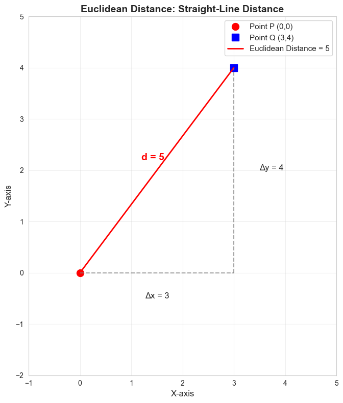

2. Manhattan Distance (L1 Distance)¶

Formula¶

Distance by traveling only horizontally or vertically. Like navigating city blocks.

d(p, q) = |p_1 - q_1| + |p_2 - q_2| + \cdots + |p_n - q_n|

(2)

Characteristics¶

Also called “taxicab distance” or “L1 norm”
You can only move up/down/left/right (no diagonals)
Often faster to compute than Euclidean
More robust to outliers

# Example: Calculate Manhattan distance
p = np.array([0, 0])
q = np.array([3, 4])

# Method 1: Manual calculation
dist_manual = np.abs(p[0] - q[0]) + np.abs(p[1] - q[1])

# Method 2: Using scipy
dist_scipy = cityblock(p, q)

print(f"Point P: {p}")
print(f"Point Q: {q}")
print(f"\nManhattan Distance (Manual): {dist_manual}")
print(f"Manhattan Distance (SciPy):  {dist_scipy}")
print(f"\nCalculation: |3-0| + |4-0| = 3 + 4 = 7")
print(f"\nCompare:")
print(f"  Euclidean:  5 (straight line)")
print(f"  Manhattan:  7 (grid path)")

Point P: [0 0]
Point Q: [3 4]

Manhattan Distance (Manual): 7
Manhattan Distance (SciPy):  7

Calculation: |3-0| + |4-0| = 3 + 4 = 7

Compare:
  Euclidean:  5 (straight line)
  Manhattan:  7 (grid path)

# Visualize Manhattan Distance
fig, (ax1, ax2) = plt.subplots(1, 2, figsize=(14, 6))

# Left: One Manhattan path
ax1.plot([0], [0], 'ro', markersize=10, label='Point P (0,0)')
ax1.plot([3], [4], 'bs', markersize=10, label='Point Q (3,4)')
ax1.plot([0, 3], [0, 0], 'g-', linewidth=3, alpha=0.7, label='Move right (3)')
ax1.plot([3, 3], [0, 4], 'b-', linewidth=3, alpha=0.7, label='Move up (4)')
ax1.text(1.5, -0.5, 'Δx = 3', fontsize=12, ha='center')
ax1.text(3.5, 2, 'Δy = 4', fontsize=12)
ax1.set_xlim(-1, 5)
ax1.set_ylim(-2, 5)
ax1.grid(True, alpha=0.3)
ax1.legend(fontsize=10)
ax1.set_title('Manhattan Distance = 7\n(One possible path)', fontsize=12, fontweight='bold')
ax1.set_aspect('equal')

# Right: Multiple Manhattan paths
ax2.plot([0], [0], 'ro', markersize=10, label='Point P (0,0)')
ax2.plot([3], [4], 'bs', markersize=10, label='Point Q (3,4)')
# Path 1: right then up
ax2.plot([0, 3, 3], [0, 0, 4], 'g--', linewidth=2, alpha=0.6)
# Path 2: up then right
ax2.plot([0, 0, 3], [0, 4, 4], 'b--', linewidth=2, alpha=0.6)
ax2.plot([0, 3], [0, 4], 'r-', linewidth=2, label='Euclidean (5)', alpha=0.8)
ax2.text(1.5, 1.5, 'All paths = 7', fontsize=12, color='green', fontweight='bold')
ax2.set_xlim(-1, 5)
ax2.set_ylim(-2, 5)
ax2.grid(True, alpha=0.3)
ax2.legend(fontsize=10)
ax2.set_title('All Manhattan Paths Have Same Distance', fontsize=12, fontweight='bold')
ax2.set_aspect('equal')

plt.tight_layout()
plt.show()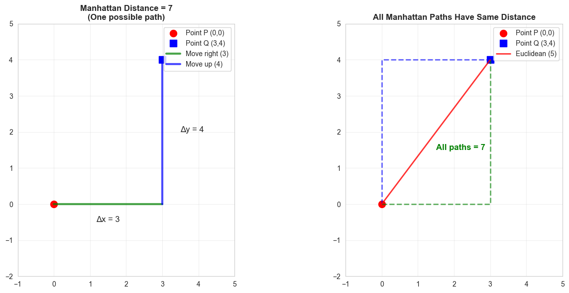

3. Minkowski Distance¶

Formula¶

A generalized distance metric that includes both Euclidean and Manhattan as special cases.

d(p, q) = \left( \sum_{i=1}^{n} |p_i - q_i|^p \right)^{1/p}

(3)

Special Cases¶

p = 1: Manhattan distance
p = 2: Euclidean distance
p = ∞: Chebyshev distance (maximum difference)

Characteristics¶

Flexible - can adjust the parameter p
p=1 emphasizes absolute differences
p=2 is most commonly used
p>2 emphasizes larger differences

# Example: Calculate Minkowski distance for different p values
p_point = np.array([0, 0])
q_point = np.array([3, 4])

print(f"Point P: {p_point}")
print(f"Point Q: {q_point}")
print(f"\nMinkowski Distance for different p values:")
print("="*50)

for p in [1, 1.5, 2, 3, np.inf]:
    if p == np.inf:
        dist = np.max(np.abs(p_point - q_point))
        print(f"p = ∞  (Chebyshev):   {dist}")
    else:
        dist = minkowski(p_point, q_point, p)
        print(f"p = {p:<3} (L{p} norm):   {dist:.4f}")

Point P: [0 0]
Point Q: [3 4]

Minkowski Distance for different p values:
==================================================
p = 1   (L1 norm):   7.0000
p = 1.5 (L1.5 norm):   5.5843
p = 2   (L2 norm):   5.0000
p = 3   (L3 norm):   4.4979
p = ∞  (Chebyshev):   4

# Visualize how p affects Minkowski distance
p_values = np.linspace(1, 5, 50)
distances = [minkowski(p_point, q_point, p) for p in p_values]

plt.figure(figsize=(10, 6))
plt.plot(p_values, distances, 'b-', linewidth=2.5)
plt.axhline(y=5, color='r', linestyle='--', linewidth=2, alpha=0.7, label='Euclidean (p=2) = 5')
plt.axhline(y=7, color='g', linestyle='--', linewidth=2, alpha=0.7, label='Manhattan (p=1) = 7')
plt.scatter([1, 2], [7, 5], s=100, c=['green', 'red'], zorder=5)

plt.xlabel('p (parameter)', fontsize=12)
plt.ylabel('Distance', fontsize=12)
plt.title('Minkowski Distance Changes with p Parameter', fontsize=14, fontweight='bold')
plt.grid(True, alpha=0.3)
plt.legend(fontsize=11)
plt.tight_layout()
plt.show()

print("Key insight: As p increases, Minkowski distance decreases toward Chebyshev distance")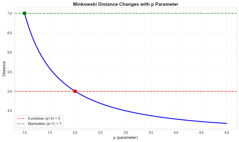

Key insight: As p increases, Minkowski distance decreases toward Chebyshev distance

4. Cosine Distance (Angle-based)¶

Formula¶

Measures the angle between two vectors, not their magnitude.

\text{Cosine Similarity} = \frac{\vec{p} \cdot \vec{q}}{\|\vec{p}\| \|\vec{q}\|}

(4)

\text{Cosine Distance} = 1 - \text{Cosine Similarity}

(5)

Characteristics¶

Values between 0 and 1 (or -1 to 1)
0 = identical direction (same angle)
1 = opposite direction
Ignores magnitude, only cares about direction
Great for text/document similarity

# Example: Calculate Cosine distance
p = np.array([1, 0])
q = np.array([1, 1])

# Method 1: Manual calculation
dot_product = np.dot(p, q)
magnitude_p = np.linalg.norm(p)
magnitude_q = np.linalg.norm(q)
cosine_sim = dot_product / (magnitude_p * magnitude_q)
cosine_dist = 1 - cosine_sim

# Method 2: Using scipy
cosine_dist_scipy = cosine(p, q)

print(f"Point P: {p}")
print(f"Point Q: {q}")
print(f"\nDot product: {dot_product}")
print(f"Magnitude of P: {magnitude_p:.4f}")
print(f"Magnitude of Q: {magnitude_q:.4f}")
print(f"\nCosine Similarity: {cosine_sim:.4f}")
print(f"Cosine Distance (Manual): {cosine_dist:.4f}")
print(f"Cosine Distance (SciPy):  {cosine_dist_scipy:.4f}")
print(f"\nInterpretation: Vectors point in similar directions (angle ≈ 45°)")

Point P: [1 0]
Point Q: [1 1]

Dot product: 1
Magnitude of P: 1.0000
Magnitude of Q: 1.4142

Cosine Similarity: 0.7071
Cosine Distance (Manual): 0.2929
Cosine Distance (SciPy):  0.2929

Interpretation: Vectors point in similar directions (angle ≈ 45°)

# Visualize Cosine Distance
fig, axes = plt.subplots(1, 3, figsize=(15, 5))

# Case 1: Similar direction (low cosine distance)
ax = axes[0]
p1, q1 = np.array([1, 0.5]), np.array([2, 1])
ax.arrow(0, 0, p1[0], p1[1], head_width=0.1, head_length=0.1, fc='red', ec='red', linewidth=2, label='Vector P')
ax.arrow(0, 0, q1[0], q1[1], head_width=0.1, head_length=0.1, fc='blue', ec='blue', linewidth=2, label='Vector Q')
cos_sim1 = cosine(p1, q1)
ax.set_xlim(-0.5, 3)
ax.set_ylim(-0.5, 2)
ax.set_aspect('equal')
ax.grid(True, alpha=0.3)
ax.legend(fontsize=11)
ax.set_title(f'Similar Direction\nCosine Distance = {1-cos_sim1:.4f}', fontsize=12, fontweight='bold')

# Case 2: Perpendicular (cosine distance = 1)
ax = axes[1]
p2, q2 = np.array([1, 0]), np.array([0, 1])
ax.arrow(0, 0, p2[0], p2[1], head_width=0.1, head_length=0.1, fc='red', ec='red', linewidth=2, label='Vector P')
ax.arrow(0, 0, q2[0], q2[1], head_width=0.1, head_length=0.1, fc='blue', ec='blue', linewidth=2, label='Vector Q')
cos_sim2 = cosine(p2, q2)
ax.set_xlim(-0.5, 1.5)
ax.set_ylim(-0.5, 1.5)
ax.set_aspect('equal')
ax.grid(True, alpha=0.3)
ax.legend(fontsize=11)
ax.set_title(f'Perpendicular (90°)\nCosine Distance = {1-cos_sim2:.4f}', fontsize=12, fontweight='bold')

# Case 3: Opposite direction (cosine distance = 2)
ax = axes[2]
p3, q3 = np.array([1, 0]), np.array([-1, 0])
ax.arrow(0, 0, p3[0], p3[1], head_width=0.1, head_length=0.1, fc='red', ec='red', linewidth=2, label='Vector P')
ax.arrow(0, 0, q3[0], q3[1], head_width=0.1, head_length=0.1, fc='blue', ec='blue', linewidth=2, label='Vector Q')
cos_sim3 = cosine(p3, q3)
ax.set_xlim(-1.5, 1.5)
ax.set_ylim(-0.5, 0.5)
ax.set_aspect('equal')
ax.grid(True, alpha=0.3)
ax.legend(fontsize=11)
ax.set_title(f'Opposite Direction (180°)\nCosine Distance = {1-cos_sim3:.4f}', fontsize=12, fontweight='bold')

plt.tight_layout()
plt.show()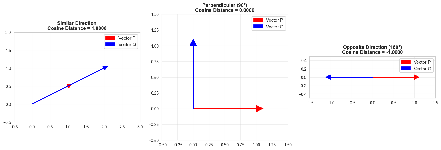

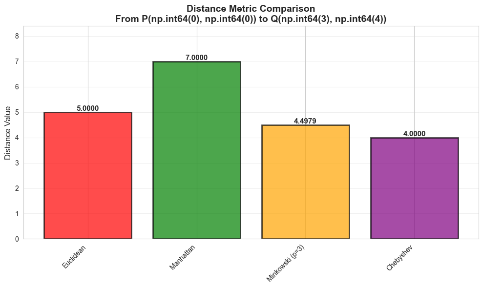
5. Comparison: All Distance Metrics¶

# Create a comparison table
p = np.array([0, 0])
q = np.array([3, 4])

metrics = {
    'Euclidean': euclidean(p, q),
    'Manhattan': cityblock(p, q),
    'Minkowski (p=3)': minkowski(p, q, 3),
    'Chebyshev': np.max(np.abs(p - q)),
    'Cosine': cosine(p, q)
}

print("\nDistance Metric Comparison")
print(f"Point P: {p}, Point Q: {q}")
print("="*50)
for metric, distance in metrics.items():
    print(f"{metric:<20} {distance:.4f}")


Distance Metric Comparison
Point P: [0 0], Point Q: [3 4]
==================================================
Euclidean            5.0000
Manhattan            7.0000
Minkowski (p=3)      4.4979
Chebyshev            4.0000
Cosine               nan

/Users/deepakkandalam/workspace/datawizard.github.io/.venv/lib/python3.9/site-packages/scipy/spatial/distance.py:647: RuntimeWarning: invalid value encountered in divide
  dist = 1.0 - uv / math.sqrt(uu * vv)

# Visual comparison
metric_names = list(metrics.keys())
metric_values = list(metrics.values())

plt.figure(figsize=(10, 6))
bars = plt.bar(metric_names, metric_values, color=['red', 'green', 'orange', 'purple', 'blue'], alpha=0.7, edgecolor='black', linewidth=2)

# Add value labels on bars
for bar, value in zip(bars, metric_values):
    height = bar.get_height()
    plt.text(bar.get_x() + bar.get_width()/2., height,
             f'{value:.4f}', ha='center', va='bottom', fontsize=11, fontweight='bold')

plt.ylabel('Distance Value', fontsize=12)
plt.title(f'Distance Metric Comparison\nFrom P{tuple(p)} to Q{tuple(q)}', fontsize=14, fontweight='bold')
plt.ylim(0, max(metric_values) * 1.2)
plt.xticks(rotation=45, ha='right')
plt.grid(True, alpha=0.3, axis='y')
plt.tight_layout()
plt.show()

posx and posy should be finite values
posx and posy should be finite values
posx and posy should be finite values

6. When to Use Each Metric¶

Metric	Best For	Pros	Cons
Euclidean	Most ML tasks, KNN	Most intuitive, works well generally	Sensitive to outliers
Manhattan	High-dimensional data, robust cases	Faster, robust to outliers	Less intuitive
Minkowski	Flexible needs, parameter tuning	Can adjust for different problems	More complex
Cosine	Text/document similarity, sparse data	Direction-based, ignores scale	Not true distance
Chebyshev	Game algorithms, grid-based problems	Fast to compute	Less common in ML

Decision Guide:¶

Default choice: Euclidean distance
Text/NLP: Cosine distance
High dimensions: Manhattan or Cosine
Need robustness: Manhattan
Grid-based problems: Chebyshev

# Real-world example: Distance between movie ratings
# User 1 rated: Action=5, Comedy=3, Drama=4
# User 2 rated: Action=5, Comedy=4, Drama=3

user1 = np.array([5, 3, 4])
user2 = np.array([5, 4, 3])

print("\n" + "="*60)
print("Real-World Example: Movie Rating Similarity")
print("="*60)
print(f"\nUser 1 ratings [Action, Comedy, Drama]: {user1}")
print(f"User 2 ratings [Action, Comedy, Drama]: {user2}")

euc_dist = euclidean(user1, user2)
cos_sim = cosine(user1, user2)

print(f"\nEuclidean Distance: {euc_dist:.4f}")
print(f"  → Ratings are {euc_dist:.2f} units apart")
print(f"  → Users have different rating patterns")

print(f"\nCosine Distance: {cos_sim:.4f}")
print(f"  → Their rating directions are very similar (cosine sim = {1-cos_sim:.4f})")
print(f"  → Both users like similar types of movies (just different ratings)")

print(f"\nConclusion:")
print(f"  → Use Euclidean if you care about magnitude of differences")
print(f"  → Use Cosine if you only care about preference direction")


============================================================
Real-World Example: Movie Rating Similarity
============================================================

User 1 ratings [Action, Comedy, Drama]: [5 3 4]
User 2 ratings [Action, Comedy, Drama]: [5 4 3]

Euclidean Distance: 1.4142
  → Ratings are 1.41 units apart
  → Users have different rating patterns

Cosine Distance: 0.0200
  → Their rating directions are very similar (cosine sim = 0.9800)
  → Both users like similar types of movies (just different ratings)

Conclusion:
  → Use Euclidean if you care about magnitude of differences
  → Use Cosine if you only care about preference direction

Summary¶

✅ Euclidean: Default choice, straight-line distance
✅ Manhattan: Grid-based, robust alternative
✅ Minkowski: Flexible generalization (p=1 → Manhattan, p=2 → Euclidean)
✅ Cosine: Angle-based, great for text/vectors

Key Takeaways:¶

Different metrics measure distance differently
Choice of metric affects KNN, clustering, and other algorithms
Euclidean is the safest default
Cosine is best for high-dimensional and text data
Always test multiple metrics for your specific problem