Goal
To understand and implement mutiple evaliation methods like accuracy,precision and recall to evalaute a classification model.
Resources
Why we need to evaluate a model ?
To Measure Performance and Fitness for Purpose: is this model any good ?
To Enable Model Selection: we can experiment with other params and select the best one.
To Estimate How Well the Model Will Generalize: since model has to work for the new data, it needs to generalize better.
To Identify Strengths and Weaknesses: identify models streangths and weaknesses.
To Build Trust and Ensure Safety: with different evaulation metrics we can build trust and ensure the model is safe. -To Guide Further Development, help us to improve the model further.
Evaluation Metrics
Confusion Matrix
Accuracy
Precision
Recall
F - Score
AUC-ROC Curve [WIP]
Confusion Matrix
a confusion matrix, also known as error matrix,is a specific table layout that allows visualization of the performance of an algorithm, typically a supervised learning one. In unsupervised learning it is usually called a matching matrix. The term is used specifically in the problem of statistical classification.
Each row of the matrix represents the instances in an actual class while each column represents the instances in a predicted class, or vice versa
Table of confusion - Basic Structure (2x2 Binary Matrix)
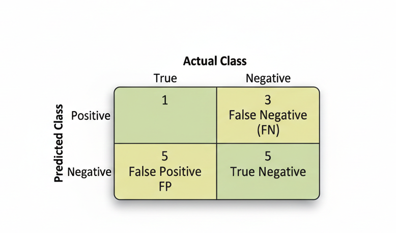
Matrix Structure
Example / Usecase
Consider we are working on the a pregnency classification model.
Consider we are working on classifying an email to be a spam or not a spam.
Actual Value
value that it not from the model,A value from data. Represented as True and False.
Predicted Value
A value predicted from model, positive - when models infers positive(yes) based on learning, negative - when models infers positive(no) based on learning.
True Positive (TP):
The model correctly predicted the positive class (e.g., correctly identified a spam email).
| Usercase | Actual <> Predicted |
|---|---|
| Spam Email text as input | Spam <> Spam |
| Women as Input | Pregnent <> Pregnent |
True Negative (TN):
The model correctly predicted the negative class (e.g., correctly identified a legitimate email).
| Usercase | Actual <> Predicted |
|---|---|
| Email(Non Spam) text as input | Email <> Email |
| Men as Input | Not Pregnent <> Not Pregnent |
False Positive (FP):
The model incorrectly predicted positive when it was actually negative (a “False Alarm” or Type I error).
| Usercase | Actual <> Predicted |
|---|---|
| Email(Non Spam) text as input | Email <> Spam |
| Men as Input | Not Pregnent <> Pregnent |
False Negative (FN):
The model incorrectly predicted negative when it was actually positive (a “Miss” or Type II error).
| Usercase | Actual <> Predicted |
|---|---|
| Spam Email text as input | Spam Email <> Email |
| Women as Input | Pregnent <> Not Pregnent |
Key Metrics Derived from the Matrix
Accuracy
Accuracy measures the total number of correct classifications divided by the total number of cases.
Where:
TP = True Positives (correct positive predictions)
TN = True Negatives (correct negative predictions)
FP = False Positives (incorrect positive predictions)
FN = False Negatives (incorrect negative predictions)
Recall/Sensitivity
Recall/Sensitivity measures the total number of true positives divided by the total number of actual positives. It answers: “Of all the actual positive cases, how many did we correctly identify?”
Also known as Sensitivity or True Positive Rate (TPR).
Precision
Precision measures the total number of true positives divided by the total number of predicted positives. It answers: “Of all the cases we predicted as positive, how many were actually positive?”
Specificity
Specificity measures the total number of true negatives divided by the total number of actual negatives. It answers: “Of all the actual negative cases, how many did we correctly identify?”
Also known as True Negative Rate (TNR).
F1 Score
F1 Score is a single metric that is a harmonic mean of precision and recall. It balances both metrics and is useful when you need a single score.
Or equivalently:
Sample by usecase
Considering the spam example, by using some synthetic data here is the sample
Spam Email Classification Example
Suppose we have a spam email classifier that was tested on 100 emails. Here’s the confusion matrix:
| Predicted Spam | Predicted Not Spam | |
|---|---|---|
| Actually Spam | 45 (TP) | 5 (FN) |
| Actually Not Spam | 10 (FP) | 40 (TN) |
Given:
TP (True Positives) = 45
TN (True Negatives) = 40
FP (False Positives) = 10
FN (False Negatives) = 5
Total = 100
Accuracy Calculation
Interpretation: The model correctly classified 85% of all emails.
Recall/Sensitivity Calculation
Interpretation: Of all the actual spam emails, the model correctly identified 90%. It missed 10% of spam emails (false negatives).
Precision Calculation
Interpretation: Of all emails the model predicted as spam, 81.8% were actually spam. There’s an 18.2% false alarm rate.
Specificity Calculation
Interpretation: Of all the actual non-spam emails, the model correctly identified 80%. It incorrectly flagged 20% as spam.
F1 Score Calculation
Interpretation: The F1 Score of 0.857 balances both precision and recall, indicating a well-performing model overall.
Summary of Results
| Metric | Value | Meaning |
|---|---|---|
| Accuracy | 85% | Overall correctness |
| Recall (Sensitivity) | 90% | Catches most spam emails |
| Precision | 81.8% | Most predicted spam are actually spam |
| Specificity | 80% | Correctly identifies legitimate emails |
| F1 Score | 85.7% | Balanced performance metric |
When to Use Each Metric
Accuracy: Use when all misclassifications have equal cost (balanced dataset)
Recall: Use when missing positive cases is costly (e.g., cancer detection - missing a patient is worse than a false alarm)
Precision: Use when false positives are costly (e.g., spam filter - incorrectly marking legitimate emails as spam is annoying)
Specificity: Use when you care about negative class identification (e.g., identifying healthy patients)
F1 Score: Use when you need a single metric balancing both precision and recall (imbalanced datasets)
Precision vs Recall
For a detailed comparison of Precision and Recall, including real-world examples and when to use each metric, see Precision vs Recall: A Detailed Comparison
Confusion Matrix using Python
Key Python Libraries
| Library | Purpose |
|---|---|
sklearn.metrics.confusion_matrix() | Create confusion matrix from predictions |
sklearn.metrics.classification_report() | Get detailed metrics report |
seaborn.heatmap() | Visualize confusion matrix as heatmap |
matplotlib.pyplot | Create plots and visualizations |
pandas.DataFrame() | Display confusion matrix in table format |
Basic Confusion Matrix Creation
Here’s how to create and visualize a confusion matrix using Python:
from sklearn.metrics import confusion_matrix, classification_report
from sklearn.model_selection import train_test_split
from sklearn.ensemble import RandomForestClassifier
import numpy as np
import pandas as pd

# Example: Spam Email Classification

# Actual labels (ground truth)
y_true = np.array([1, 0, 1, 1, 0, 1, 0, 0, 1, 1])

# Predicted labels (from your model)
y_pred = np.array([1, 0, 1, 0, 0, 1, 0, 1, 1, 1])

# Create confusion matrix
cm = confusion_matrix(y_true, y_pred)

print("Confusion Matrix:")
print(cm)
# Output:
# [[5 1]
#  [1 3]]
Interpreting the Output:
Confusion Matrix:
[[5 1]
 [1 3]]

Position [0,0] = 5  → True Negatives (TN)
Position [0,1] = 1  → False Positives (FP)
Position [1,0] = 1  → False Negatives (FN)
Position [1,1] = 3  → True Positives (TP)
Create Confusion Matrix as DataFrame
# Create a more readable confusion matrix using pandas

cm = confusion_matrix(y_true, y_pred)
cm_df = pd.DataFrame(cm,
                     index=['Actually Negative', 'Actually Positive'],
                     columns=['Predicted Negative', 'Predicted Positive'])

print(cm_df)

#                    Predicted Negative  Predicted Positive
# Actually Negative                   5                   1
# Actually Positive                   1                   3
Calculate Metrics from Confusion Matrix
from sklearn.metrics import accuracy_score, precision_score, recall_score, f1_score

# Calculate all evaluation metrics
accuracy = accuracy_score(y_true, y_pred)
precision = precision_score(y_true, y_pred)
recall = recall_score(y_true, y_pred)
f1 = f1_score(y_true, y_pred)

print(f"Accuracy:  {accuracy:.2%}")
print(f"Precision: {precision:.2%}")
print(f"Recall:    {recall:.2%}")
print(f"F1 Score:  {f1:.2%}")

# Output:
# Accuracy:  80.00%
# Precision: 75.00%
# Recall:    75.00%
# F1 Score:  75.00%
Visualize Confusion Matrix with Heatmap
import matplotlib.pyplot as plt
import seaborn as sns

# Create confusion matrix
cm = confusion_matrix(y_true, y_pred)

# Create heatmap
plt.figure(figsize=(8, 6))
sns.heatmap(cm,
            annot=True,          # Show numbers in cells
            fmt='d',              # Format as integers
            cmap='Blues',         # Color scheme
            xticklabels=['Negative', 'Positive'],
            yticklabels=['Negative', 'Positive'],
            cbar_kws={'label': 'Count'})

plt.title('Confusion Matrix - Spam Email Classification', fontsize=14, fontweight='bold')
plt.ylabel('Actual Class', fontsize=12)
plt.xlabel('Predicted Class', fontsize=12)
plt.tight_layout()
plt.show()
Output Visualization:
Confusion Matrix - Spam Email Classification

            Negative  Positive
Negative      5         1
Positive      1         3
Common Scenarios
Scenario 1: Binary Classification (2 Classes)
# Spam vs Not Spam
y_true = [0, 1, 1, 0, 1, 0, 0, 1]
y_pred = [0, 1, 0, 0, 1, 0, 1, 1]

cm = confusion_matrix(y_true, y_pred)
# Works perfectly with 2x2 matrix
Scenario 2: Multi-class Classification (3+ Classes)
# Email categories: Spam, Promotions, Important
y_true = [0, 1, 2, 0, 1, 2, 0, 1]
y_pred = [0, 1, 1, 0, 1, 2, 0, 2]

cm = confusion_matrix(y_true, y_pred)
# Creates 3x3 confusion matrix
print(cm.shape)  # (3, 3)
Tips for Working with Confusion Matrices
Always check total samples: Sum of all values should equal total test set size
Normalize for comparison: Divide by row totals to see percentages
Use classification_report(): Provides precision, recall, and F1 for each class
Visualize before analyzing: Heatmaps make patterns obvious
Check for class imbalance: If one class dominates, consider accuracy alternatives